Raw-materials simulator — Patricio Contreras Pardo

The problem

A mining company moves raw material by truck from several sources to its plant. Tracking those movements and planning transport depended on manual records and a spreadsheet.

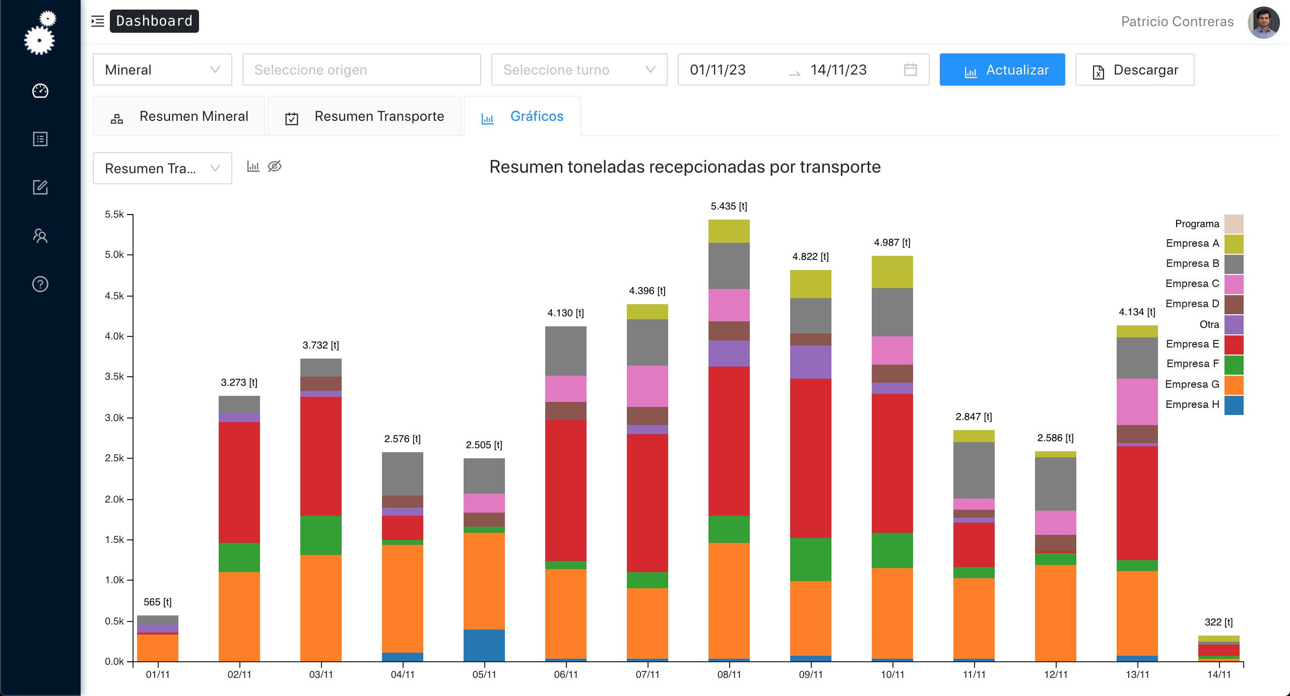
The client needed to track movements, follow them on a dashboard, export reports, and generate a feasible transport plan from historical data. The system also had to run 24/7 at a remote site with a slow internet connection.

I was the tech lead. I worked directly with the client through meetings and prototype reviews, agreed scope and priorities with the project managers, designed the database, and wrote most of the code for the frontend, the backend, and the optimizer.

From requirements to a working system

After the first meetings I designed the relational model and built a prototype, so the client could check the requirements before the full application existed. Once the system was running, each period's deliveries became the data for planning the next one.

Operating loop from dispatch to the next plan

Each movement is recorded when it leaves a source and again when it arrives at the plant. The API rejects records that would corrupt that history, such as duplicates or an arrival before its departure.

System design

The frontend, backend, and report generator deploy independently, and the optimizer runs inside the backend process. The frontend calls the backend over REST.

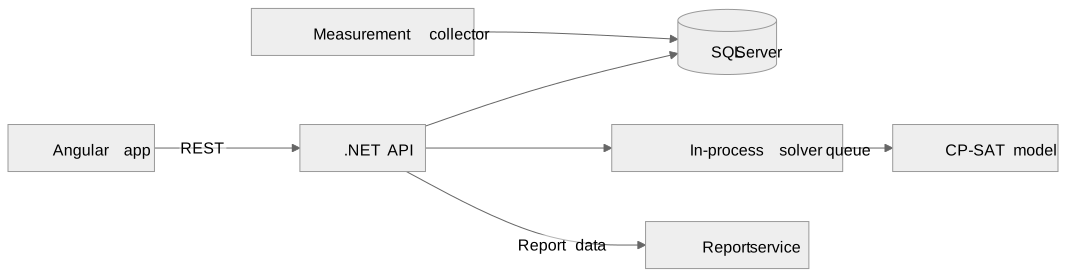
The same backend build runs as a Windows service or in Docker, on a local server or on AWS. Users sign in with tokens and integrations use API keys. Every endpoint checks the caller's role, and revoking a key also invalidates the tokens issued under it.

A second module on the same backend collects plant measurements on a schedule. It fills gaps after an outage and raises alerts when readings look wrong.

Learning parameters from history

The simulator estimates how much a truck carries and how many trips it makes from a recent window of receptions. For source $j$ and carrier $k$ , with $L_{jk}$ in tonnes per trip:

L_{jk} = \operatorname{median}\big(\text{received weight per trip}\big), \qquad R_{jk} = \operatorname{mode}\big(\text{trips per truck per day}\big)

An unusual trip barely moves the median, and the mode gives a whole number of trips. A source and carrier pair with no history gets no parameters. If a source has no usable pairs, the run leaves it out and warns the planner.

The fleet of carrier $k$ on day $d$ is $C_{kd}$ . It is the number of trucks the planner declared available that day or, if none were declared, the trucks the carrier used in the history window.

The model

A scenario covers a date range, with planned tonnes per source per day and, optionally, available trucks per carrier per day.

Sets and parameters. $D$ is the set of days, $J$ the sources with planned tonnage, and $K$ the carriers with at least one source that has history. $q_{jd}$ is the tonnage planned at source $j$ on day $d$ . CP-SAT needs integer coefficients, so tonnes become kilograms:

a_{jk} = \big\lfloor 1000 \, L_{jk} \, R_{jk} \big\rfloor, \qquad b_{jd} = \big\lfloor 1000 \, q_{jd} \big\rfloor

$a_{jk}$ is what one truck of carrier $k$ moves from source $j$ in a day.

Decision variables. $x_{djk}$ is the number of trucks carrier $k$ sends to source $j$ on day $d$ . It can be positive only when the source has tonnage that day and the pair has history, up to a bound $U$ :

x_{djk} \in \mathbb{Z}, \qquad 0 \le x_{djk} \le \begin{cases} U & \text{if } q_{jd} > 0 \text{ and } a_{jk} > 0 \\ 0 & \text{otherwise} \end{cases}

Cover the plan. The trucks sent to a source must move at least its planned tonnes:

\sum_{k \in K} a_{jk} \, x_{djk} \ge b_{jd} \qquad \forall d \in D,\ j \in J

Respect each fleet. A carrier cannot send more trucks than it has that day:

\sum_{j \in J} x_{djk} \le C_{kd} \qquad \forall d \in D,\ k \in K

Objective. Use as few truck-days as possible:

\min \sum_{d \in D} \sum_{j \in J} \sum_{k \in K} x_{djk}

Every truck-day costs the same, so the solver prefers carriers that have moved more tonnes per truck per day at a source. When a carrier loads more or completes more trips, its $a_{jk}$ rises, and the solver can assign it more trucks in the next scenario. CP-SAT solves the model under a time limit with parallel search workers.

Why the search space is large

Count only the ways one carrier can spread its fleet on one day. With $C$ trucks, $n$ sources, and idle trucks allowed, stars and bars gives:

N(C, n) = \binom{C + n}{n}

Take a hypothetical operation with 5 sources and 4 carriers of 10 trucks each. One carrier has $\binom{15}{5} = 3003$ ways to place its trucks on a day, the four carriers together have $3003^4 \approx 8.1 \times 10^{13}$ , and a 30-day scenario has about $10^{417}$ plans before any coverage check. No constraint links two days, so the model splits into one independent problem per day. Within a day, CP-SAT propagates the coverage and fleet bounds to prune most of those combinations.

Running the solver without blocking the API

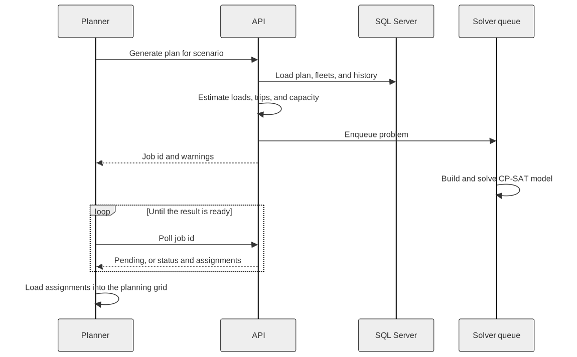
A solve can run until its time limit, longer than a web request should wait. The API puts each problem on an in-process queue and returns a job id. A background consumer solves one model at a time and keeps the result in memory.

From solution to published plan

Planners work in scenarios they can copy, resize, and reload with new plan or fleet data. The solution opens in an editable grid with trucks, load, and trips for each source and carrier by day, next to the gap between the resulting tonnes and the plan. Planners can change any value or add and remove carriers. A carrier added by hand starts with its historical load and trips.

Publishing freezes a copy of the plan for a date range, so later scenario edits leave it unchanged. The system warns before a publication overlaps an earlier one and notifies the people who follow the plan.

Tracking the plan against receptions

The dashboard and reports compare the published plan with what the plant received, by day, week, or month. For carrier $k$ over a period, let $x_{djk}$ , $r_{djk}$ , and $\ell_{djk}$ be the trucks, trips per truck, and load per trip in the published plan. These start from the solution and historical values, and planners may have edited them. On the reception side, $T_k$ is the tonnes received, $\hat{x}_k$ the truck-days with arrivals (a truck counts once per day), and $\hat{\ell}_k$ the average received weight per trip. The planned tonnes $P_k$ and the tracking metrics are:

P_k = \sum_{d,j} x_{djk} \, r_{djk} \, \ell_{djk}, \qquad \text{coverage}_k = 100 \, \frac{\hat{x}_k}{\sum_{d,j} x_{djk}}, \qquad \text{progress}_k = 100 \, \frac{T_k}{P_k}, \qquad \hat{r}_k = \frac{T_k}{\hat{x}_k \, \hat{\ell}_k}

Coverage tells planners whether a carrier sent the trucks it was assigned, progress tells them whether those trucks moved the tonnes, and $\hat{r}_k$ is the trips actually made per truck-day. Cycle time is the average time between consecutive arrivals of the same truck on the same day.

Excel reports come from a separate Node.js service. The API reuses the summaries behind its screens, sends them to the service as JSON, and returns the workbook. If the service is down, the rest of the application keeps working.

Trade-offs

Fewest trucks as the objective

Minimizing truck-days keeps the model linear and answers the spreadsheet's question of how many trucks each carrier sends where. Integer trucks can overshoot the plan, and the grid shows planners by how much.

Learned loads and trips instead of declared ones

Because loads and trips come from receptions, the plan follows what carriers actually did. The solver never sends a carrier to a source where it has no history, although planners can add that carrier by hand.

Hard coverage

Every source must reach its planned tonnes every day. If the fleets cannot cover a day, the model is infeasible and the planner gets no plan. The planner can declare more trucks or change the plan and run it again.

An in-process solver

Solving inside the API keeps deployment to one service at a remote site. In exchange, jobs run one at a time and results do not survive a restart.

Delivery

The system went into production and was deployed on AWS in 2022.

What I brought to it

The project started from high-level requirements. Working directly with the client, I shaped them into a data model and a prototype we reviewed together, and then into a production system with operational screens, a dashboard, reports, and an optimizer.

On the planning side, I turned the spreadsheet's carrier assignment into an integer model whose parameters come from the operation's own receptions, so each new plan reflects how carriers have recently performed.