Packaging batch optimizer — Patricio Contreras Pardo

The problem

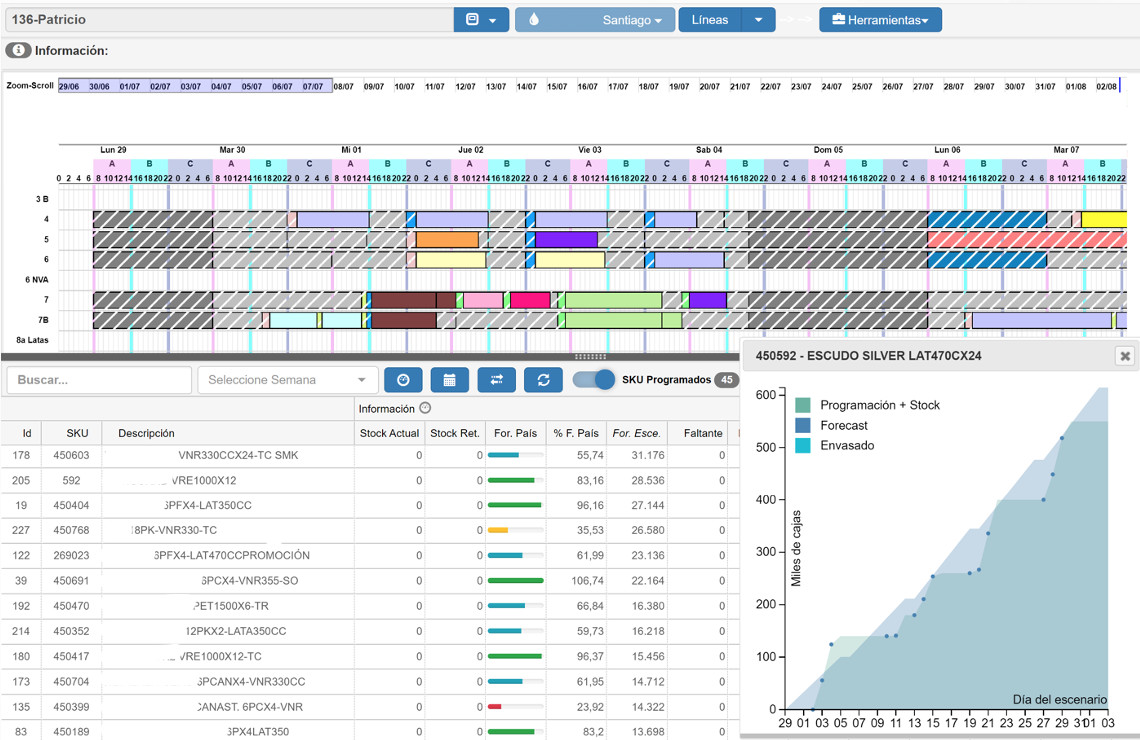
A beverage producer schedules production on its packaging lines. Planners schedule ahead and refine each week's plan as it approaches. The unit of work is a batch: a product and a quantity. For every batch, the plan decides which line runs it, in what order, and when.

Planning cycle from the forward plan to the weekly schedule

A plan has to respect all of these inputs at once:

Each line runs each product at its own actual and nominal rate, and some lines cannot run some products.
Switching products costs setup time, which each line defines in its own changeover matrix.
Downtime, shift windows, and start-up calendars remove time from each line.
Some batches have a minimum lot size, so a line cannot run a small piece of them.
Stock and daily forecasts set how soon each product is needed.

The client measures lines with an efficiency KPI in the family of overall equipment effectiveness (OEE): theoretical work time divided by effective work time. Theoretical time is good output divided by nominal speed, so a slower line has a higher effective time and a lower score. If a line runs $q$ units at an actual rate $y$ against a nominal rate $\bar{y}$ :

t = \frac{q}{y}, \qquad t_{\text{theoretical}} = \frac{q}{\bar{y}} = t \cdot \frac{y}{\bar{y}}, \qquad \eta = \frac{\sum t_{\text{theoretical}}}{\sum t_{\text{effective}}}

Effective time counts everything the line spends on the plan: batch time, changeovers, idle gaps between batches, and the delay before the first batch starts. Efficiency goes up when each product runs on the line closest to its nominal speed and batches are ordered to keep changeovers short.

The existing optimizer used simulated annealing, built its problem from a mix of SQL queries, T-SQL stored procedures, and .NET code, and ran on the application server. I led the replacement from the initial client requirements through delivery.

Why the search space explodes

Leave time aside and count only which line runs each batch and in what order. With $n$ batches and $m$ lines, a schedule splits the batches into $m$ ordered sequences, and some sequences can be empty. Assignment alone allows up to $m^n$ options. Ordering each line multiplies that:

N(n, m) = n! \binom{n+m-1}{m-1} = \frac{(n+m-1)!}{(m-1)!}

Take a small hypothetical case of 20 batches on 4 lines. It has about $1.1 \times 10^{12}$ assignments and $4.3 \times 10^{21}$ ordered schedules. Checking a billion schedules per second would take about 136,000 years. Start times, shift windows, and partial runs make the real space larger.

CP-SAT cuts the space down with constraint propagation, clause learning, and linear relaxations. It runs several search strategies in parallel and returns the best plan found when the time limit ends.

Three model versions

The model changed as the client added rules.

Version	What changed
v1 (2021)	One integer model assigns and sequences batches against each line's capacity in hours.
v2 (2023)	CP-SAT with time intervals. Downtime, shift windows, and calendars become constraints. A second stage cuts batches into shift windows, and stock coverage enters the objective.
v3 (2024)	Partial and left-out batches carry penalties, and efficiency becomes a linear objective. Minimum lot applies per batch, the cutter runs on every line that has shift windows, and stock shortages become alerts. v3 went into production.

System design

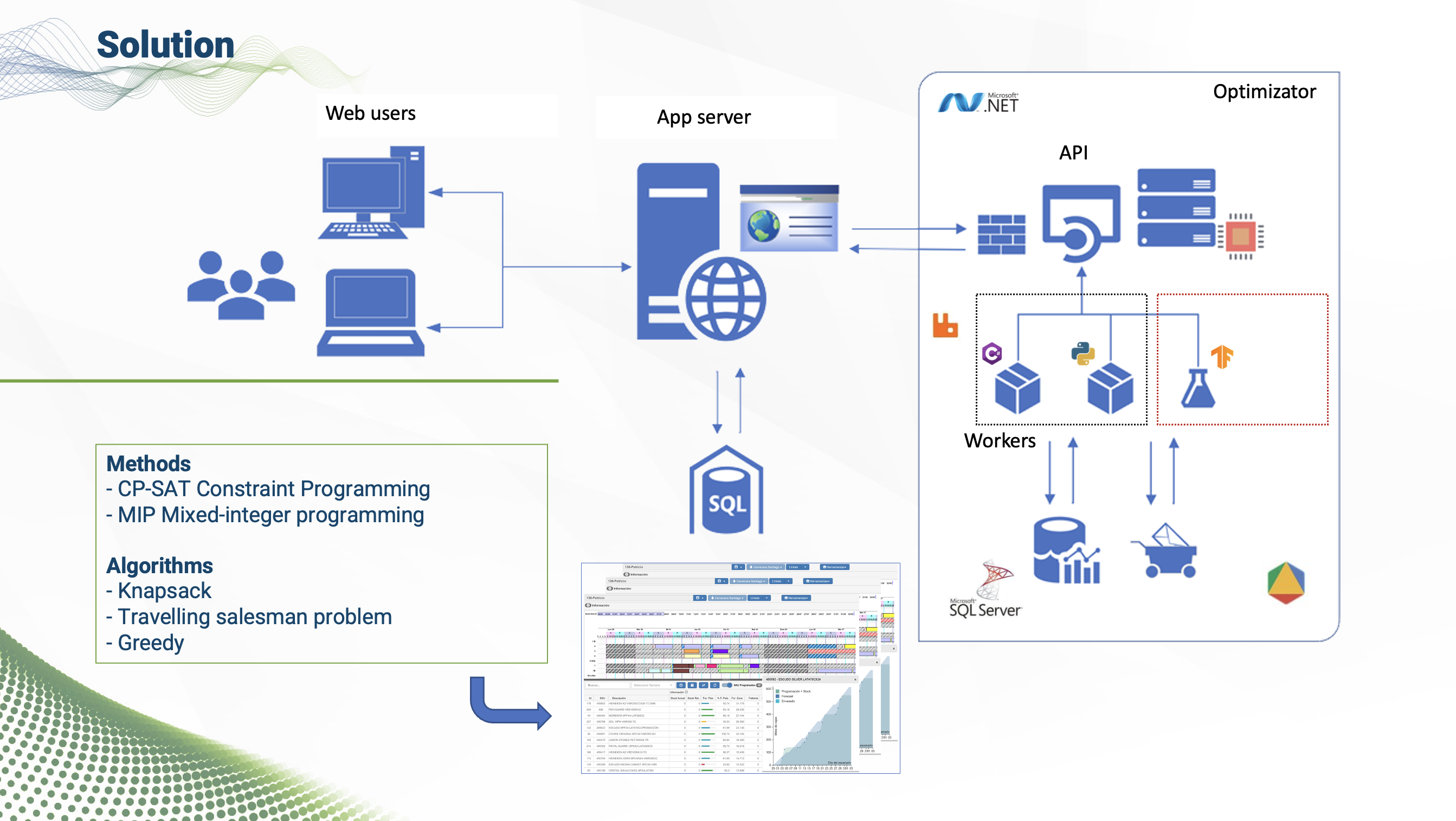
I moved optimization off the application server into separate services. A .NET Core and Entity Framework API owns the jobs in SQL Server, and solver workers take jobs from RabbitMQ. The application and the optimizer deploy independently, and the workers first ran on AWS.

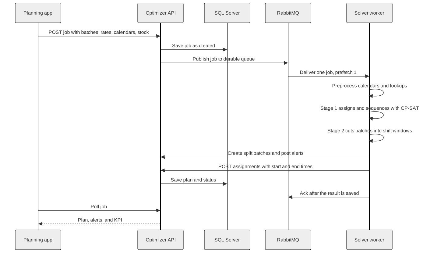
Job lifecycle from planning request to saved plan

Each worker sets a prefetch of 1, so it holds one job at a time and gives the solver all of its configured cores. Adding capacity means adding worker instances.

The worker acknowledges a message only after it posts the result. If a worker stops mid-solve, RabbitMQ delivers the job again. The API also writes each incoming job as JSON before queueing it, so any plan can be solved again from the same input.

Preparing the model input

Before building a model, the worker normalizes time. Overlapping downtime on a line merges into one event. Downtime is subtracted from shift windows, and a window that loses its middle splits in two. Each line's available time is the sum of what remains, and day boundaries start at the first midnight in the planning range.

CP-SAT works with integers. Batch lengths rounded to whole minutes lost output, so the model counts time in hundredths of a minute, with a scale factor $A = 100$ . With rates in units per hour, the length of batch $j$ on line $i$ is:

p_{ij} = \left\lfloor \frac{60 \, A \, q_j}{y_{ij}} \right\rfloor

Each job carries these settings:

Parameter	Meaning
Model	Assignment only, sequencing for one line, or the full model.
Objective	Maximize efficiency, minimize production time, or minimize total span.
Time limit	A deadline per job, with a worker default.
Search workers	CP-SAT parallel search workers, set from the host's configured cores.
Time scale	$A$ integer units per minute.
Stock targets	The level each product should hold in each period.
Flags	Include downtime and apply minimum lot.

Stage 1: assign and sequence

One CP-SAT model covers every line.

Sets and parameters. $L$ is the set of lines, $J$ the set of batches, $J_g \subseteq J$ the batches of product $g$ , and $E_{ir}$ the downtime intervals on line $i$ . Batch $j$ has quantity $q_j$ and minimum lot $b_j$ . Line $i$ runs batch $j$ at actual rate $y_{ij}$ and nominal rate $\bar{y}_{ij}$ . Changing from batch $j$ to batch $k$ on line $i$ takes $c_{ijk}$ minutes. $H_i$ is the line's horizon, based on its available time.

Decision variables. A variable exists only when $y_{ij} > 0$ , so an ineligible line never appears in the model.

$x_{ij} \in \{0,1\}$ is 1 when line $i$ runs batch $j$ .
$s_{ij}, e_{ij} \in [0, H_i]$ are its start and end. They form an optional interval $I_{ij}$ , at most $p_{ij}$ long, that exists only when $x_{ij} = 1$ .
$u_j \in \{0,1\}$ is 1 when batch $j$ is left out.
$\ell_{ijk} \in \{0,1\}$ is 1 when batch $k$ directly follows batch $j$ on line $i$ . It controls an optional changeover interval $C_{ijk}$ of length $A\,c_{ijk}$ that ends when batch $k$ starts.
$\delta_{ijk} \ge 0$ is the idle gap before that changeover, and $w_{ij} \ge 0$ is the delay before a first batch.

An interval can be shorter than $p_{ij}$ , so a batch can run partially. The objective charges for that.

Assignment. Each batch runs on exactly one line or is left out:

\sum_{i \in L \,:\, y_{ij} > 0} x_{ij} + u_j = 1 \qquad \forall j \in J

Timing and no overlap. An unassigned batch has zero start and end. On each line, batches, downtime, and changeovers cannot overlap:

\begin{aligned} x_{ij} = 0 &\;\Rightarrow\; s_{ij} = e_{ij} = 0 \\ x_{ij} = 1 &\;\Rightarrow\; s_{ij} < e_{ij} \le s_{ij} + p_{ij} \\ \operatorname{NoOverlap}&\big(\{I_{ij}\}_{j} \cup \{E_{ir}\}_{r} \cup \{C_{ijk}\}_{j,k}\big) \qquad \forall i \in L \end{aligned}

Sequencing. The order on a line is a Hamiltonian path. CP-SAT's circuit constraint expresses it with a dummy depot node 0. An arc from the depot marks the first batch, and an arc back to it marks the last. A self-loop on node $j$ means the line skips that batch. The depot has no self-loop, so every line in the model runs at least one batch.

\operatorname{Circuit}_i\Big( \{(0 \to j,\ \ell_{i0j})\} \cup \{(j \to 0,\ \ell_{ij0})\} \cup \{(j \to j,\ 1 - x_{ij})\} \cup \{(j \to k,\ \ell_{ijk})\} \Big)

Each arc is tied to the timeline. A chosen arc forces its changeover time, and the model records the idle gap and the delay before the first batch:

\begin{aligned} \ell_{ijk} = 1 &\;\Rightarrow\; e_{ij} + A\,c_{ijk} \le s_{ik} \\ \ell_{ijk} = 1 &\;\Rightarrow\; \delta_{ijk} = s_{ik} - A\,c_{ijk} - e_{ij} \\ \ell_{i0j} = 1 &\;\Rightarrow\; w_{ij} = s_{ij} \\ \ell_{ijk} &\le x_{ij}, \quad \ell_{ijk} \le x_{ik} \end{aligned}

Minimum lot. If a batch runs at all, it runs long enough to make its minimum lot:

x_{ij} = 1 \;\Rightarrow\; e_{ij} - s_{ij} \ge \left\lfloor \frac{60 \, A \, b_j}{y_{ij}} \right\rfloor

Objective. The v3 prototype first stated efficiency as a ratio minus penalties. CP-SAT needs a linear objective, and the revision minimizes the difference between effective and theoretical time. Theoretical time uses $\rho_{ij} = \lfloor A\,y_{ij}/\bar{y}_{ij} \rfloor$ , so the other terms are also multiplied by $A$ to stay on the same scale:

\begin{aligned} \min \;\; & A \underbrace{\Big[\sum_{i,j} (e_{ij} - s_{ij}) + \sum_{i,j,k} \big(A\,c_{ijk}\,\ell_{ijk} + \delta_{ijk}\big) + \sum_{i,j} w_{ij}\Big]}_{\text{effective time}} - \underbrace{\sum_{i,j} \rho_{ij}\,(e_{ij} - s_{ij})}_{\text{theoretical time}} \\ & + A \underbrace{\sum_{i,j} \big(p_{ij}\,x_{ij} - (e_{ij} - s_{ij})\big)}_{\text{partial runs}} + A \underbrace{\sum_{j} u_j \max_{i} p_{ij}}_{\text{left out}} \end{aligned}

Batch time and the partial-run penalty add up to $A\,p_{ij}\,x_{ij}$ . Every assigned batch pays for its full length and earns back $\rho_{ij}$ for each unit of time it actually runs. A batch left out costs its longest possible run time, so the solver drops it only when that lowers the total.

Stock coverage

A schedule can look efficient and still let a product run out. The model projects stock for each product $g$ over each period $d$ of the horizon. Production placed in the period adds to stock, and forecast demand $F_{gd}$ draws it down. A shortage is how far stock plus production falls below a target $\bar{S}_{gd}$ , and the target already accounts for the period's demand:

\begin{aligned} P_{gd} &= \sum_{i,\,j \in J_g} \frac{q_j}{p_{ij}} \,\big\lvert [s_{ij}, e_{ij}) \cap \text{period}_d \big\rvert \\ S_{g,d+1} &= \max\big(0,\ S_{gd} + P_{gd} - F_{gd}\big) \\ \sigma_{gd} &= \max\big(0,\ \bar{S}_{gd} - (S_{gd} + P_{gd})\big) \end{aligned}

$P_{gd}$ counts what the batches of product $g$ produce during the part of their intervals that falls in period $d$ . The shortage is a soft constraint: v2 adds $\sum \omega_{gd}\,\sigma_{gd}$ to the stage 1 objective, with weights that put it on the same scale as time and make early shortages cost more. v3 drops the term from the objective and reports shortages as alerts.

Stage 2: cutting batches into shift windows

Stage 1 places each batch as one block, but a line with shift windows can only run inside them, so a long batch has to be split. The cutter is a fractional knapsack across several windows, written in CP-SAT and run per line. Its bins are shift windows with downtime removed, and its items are the batches stage 1 put on that line.

Parameters and variables. Window $h$ has capacity $K_h$ . Batch $j$ has length $p_j$ , the time stage 1 assigned to it, and a minimum lot that takes $\mu_j$ time units. $c_{jk}$ is the line's changeover time from batch $j$ to batch $k$ .

$z_{hj} \in [0, p_j]$ is the time of batch $j$ placed in window $h$ .
$a_{hj} \in \{0,1\}$ is 1 when part of batch $j$ is in window $h$ .
$\ell_{hjk}$ is an arc literal for a circuit that orders batches inside window $h$ .

The constraints keep pieces consistent with their batch and their window:

\begin{aligned} a_{hj} = 0 &\;\Rightarrow\; z_{hj} = 0 && \text{no piece, no time} \\ a_{hj} = 1 &\;\Rightarrow\; z_{hj} \ge \mu_j && \text{each piece meets the minimum lot} \\ \sum_{h} z_{hj} &\le p_j && \text{pieces add up to at most the batch} \\ \sum_{j} z_{hj} + \sum_{j,k} A\,c_{jk}\,\ell_{hjk} &\le K_h && \text{window capacity, changeovers included} \\ a_{h-1,j} \wedge a_{hj} &\;\Rightarrow\; \ell_{h0j} = 1 && \text{a continued piece opens the next window} \end{aligned}

The pieces of one batch also have to sit in consecutive windows, and empty windows form a single block at the start or end of the horizon.

Objective. The cutter minimizes unused capacity, extra batches per window, changeovers, and time left unassigned. Each batch in a window beyond the first costs a fixed fraction $\lambda$ of that window's capacity:

\min \sum_{h} \Big(K_h - \sum_{j} z_{hj}\Big) + \sum_{h} \Big(\sum_{j} a_{hj} - 1\Big) \lambda K_h + \sum_{h,j,k} A\,c_{jk}\,\ell_{hjk} + \sum_{j} \Big(p_j - \sum_{h} z_{hj}\Big)

Unused capacity and unassigned time both shrink as more of each batch is placed, so together they push the cutter to fill windows. An empty window pays its full capacity as unused time and gets $\lambda K_h$ back from the count term.

When the cutter splits a batch, the worker creates the new batches through the API. It posts an alert for each batch that ran partially or not at all, and for each shift window left unfilled.

A test case produced the empty-window rule. The first version filled capacity but alternated used and unused days. Planners expected the unused shifts grouped together, because those groups define the available ranges. The next version added the block constraint.

Trade-offs

Which objective to optimize

In v1 we compared two objectives on the same test week. Maximizing efficiency gave a higher KPI than minimizing production time, but it scheduled more production hours and took longer to solve. Efficiency was the client's KPI, so it became the default, and v3 uses only efficiency.

Capacity buckets or intervals

v1 treated each line as a bucket of hours. That was enough to assign and sequence batches. It could not place a batch around downtime or a shift, and it could not simulate individual days. v2 moved to time intervals, which made calendars, shift windows, and daily stock possible.

One model or stages

Cutting runs as its own stage after assignment and sequencing. Stage 1 plans against each line's total available time and ignores shift boundaries, which keeps the whole-plant model smaller. Stage 2 then solves one small model per line. In exchange, each batch stays on the line stage 1 chose: the cutter can reorder batches inside a window but cannot move one to another line. If it finds no valid split, the job reports the plan as infeasible.

Hard or soft assignment

Early models required every batch to run: $\sum_i x_{ij} = 1$ . When demand exceeded available time, the model was infeasible and planners got no plan. The rule was relaxed to $\sum_i x_{ij} \le 1$ , and v3 then priced partial and missing batches in the objective. A batch that does not fit now shows up in an alert.

Simulations and testing

Planners call a scenario run a simulation, and each simulation is one job.

Unit tests run the cutter on small hand-built cases with known window capacities and changeover matrices. Some cases have more than one optimal answer: a batch that needed two of three windows came back in the first two in one run and in the last two in another.

When a plan looked wrong, we saved the job JSON under a name that described the behavior and replayed it against new builds. Those files included a shift window that ended past the horizon and a minimum lot that dropped a small piece.

Each job runs under a time limit, and a job can set its own deadline. Full-plant test runs showed where the default limit was too short.

During rollout, planners reviewed scenarios with us every week. We compared actual weeks with the optimizer's plan and checked changeover and rate data against recent history.

Delivery

Optimizer v1 improved the efficiency KPI by up to 2% over the previous optimizer. The optimizer also helped planners extend their planning horizon. The distributed system replaced the existing optimizer at the client's plants, and v3 later went into production.

What I brought to it

I have enjoyed optimization problems since college, and I like them most when the model has to answer to a real business. On this project I worked across the system, the model, and the business: I moved optimization onto queue-driven workers, designed the CP-SAT models, and turned the plant's efficiency KPI into a linear objective the solver could use.

I ran the client meetings and took the work past the original scope. The first version had two objectives, and on our own initiative we added a third that reduced the time and resources each optimization run needs.